Stab-Element R2

Video

../../../_images/R2_all.png

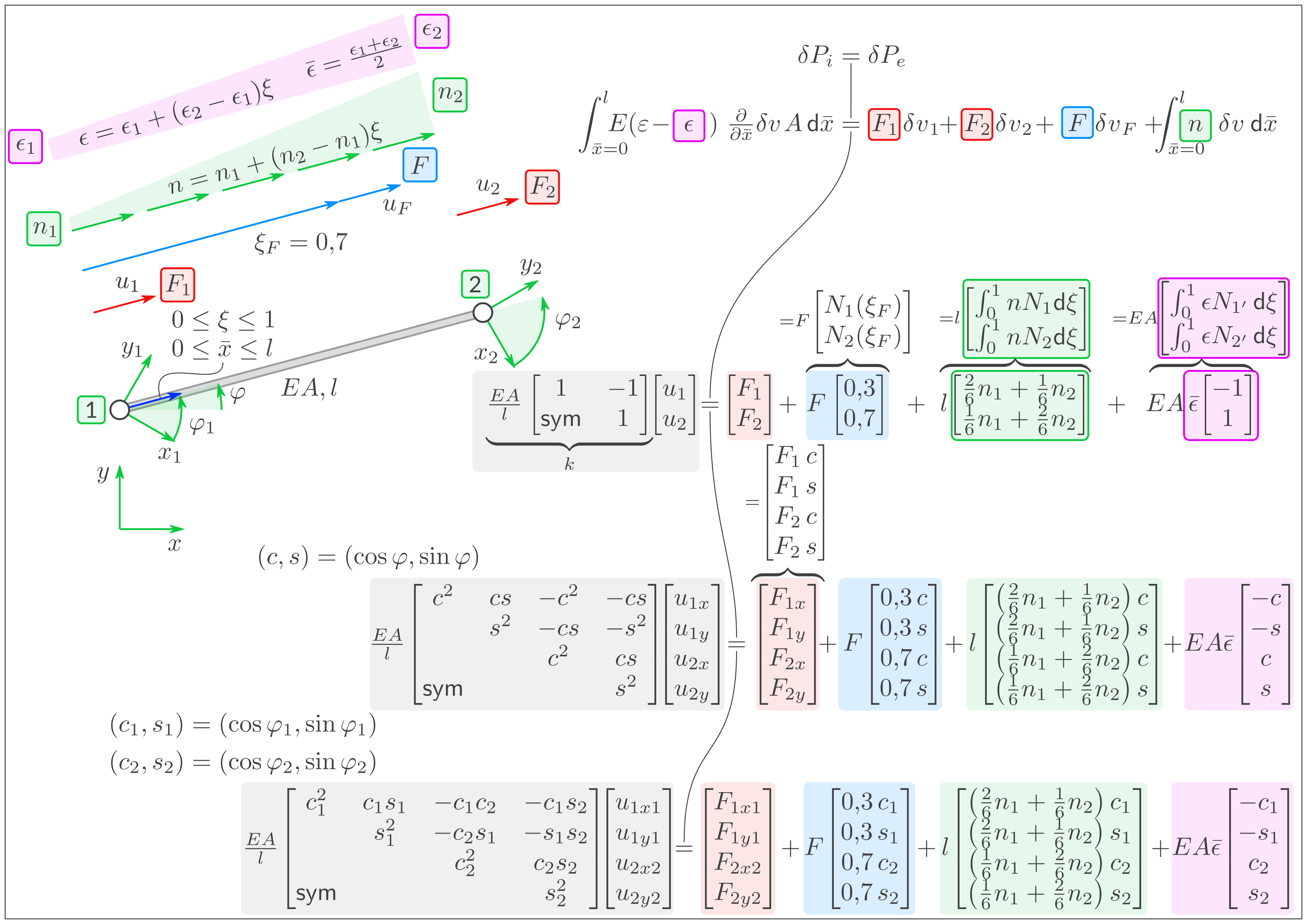
2-Knoten-Stab-Element: Prinzip der virtuellen Leistung. Äußere Lasten: Einzel-Kräfte \(F_1\) und \(F_2\) an den Knoten, Einzelkraft \(F\) zwischen den Knoten, verteilte Kraft \(n\) und Wärmeausdehnung (Verzerrung aufgrund Temperaturzuwachs) \(\epsilon\) . Lineares System in 1D und in 2D. Verwendung von \((x,y)\)-Bezugssystem bzw. von \((x_1, y_1)\)- und \((x_2, y_2)\)-Bezugssystem.

Bezeichnungen

  • \((x,y)\): Bezugssystem.

  • \((\boldsymbol u_1, \boldsymbol u_2)\): Knotenverschiebungen.

  • \(S\): Stabkraft: Wie üblich definiert, so dass für einen Zugstab gilt: \(S>0\).

  • \((\boldsymbol F_1, \boldsymbol F_2)\): Resultierende der Kräfte am Knoten (abgesehen von \(S\)).

Stab mit Winkelposition \(\varphi\):

  • \(\boldsymbol e\): Einheitsvektor in Stabrichtung: Vom ersten Knoten 1 zum zweiten Knoten 2.

  • Zählrichtung der Winkelposition \(-180^\circ < \varphi \le 180^\circ\): Positiv um die \(z\)-Achse.

  • Nullpunkt der Winkelposition: Es gilt \(\varphi=0\), falls \(x\) und \(\boldsymbol e\) deckungsgleich sind.

Merksatz: Man müsste die \(x\)-Achse um \(\varphi\) drehen, so dass sie deckungsgleich wäre mit \(\boldsymbol e\).

Für den Sonderfall, dass es Lokale Bezugssysteme gibt, gilt:

  • Es gibt zwei Winkel, nämlich \(-180^\circ < \varphi_1, \varphi_2\le 180^\circ\).

  • Es gibt zwei Bezugssysteme, nämlich \((x_1, y_1)\) und \((x_2, y_2)\).

  • Nullpunkt 1: Es gilt \(\varphi_1=0\), falls \(x_1\) und \(\boldsymbol e\) deckungsgleich sind.

  • Nullpunkt 2: Es gilt \(\varphi_2=0\), falls \(x_2\) und \(\boldsymbol e\) deckungsgleich sind.

Geometrie und Material:

  • \((l, \Delta l)\): (Stablänge undeformiert, Stabverlängerung).

  • \((E, A)\): (Elastiztätsmodul des Stab-Materials, Querschnittsfläche).

Interpolation

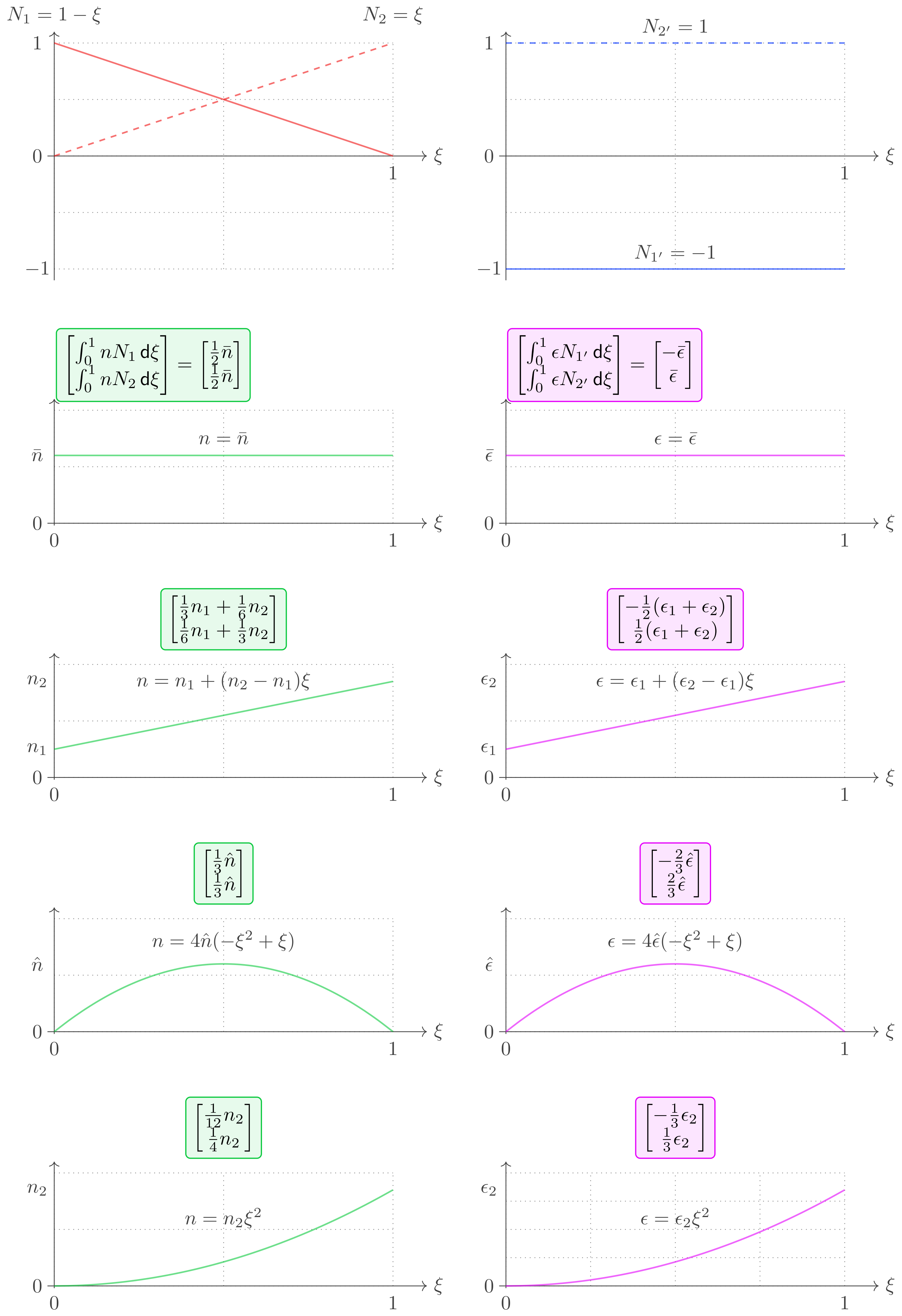
Als Ansatzfunktionen, also zur Interpolation, werden folgende Lagrange-Polynome mit der Abkürzung \(\xi = \tfrac{\bar{x}}{l}\) verwendet.

Ansatzfunktionen

\begin{align} \label{eq-R2_L} N_1 &= 1 - \left[ \tfrac{\bar{x}}{l} \right] = 1 - \xi \tag{L1}\\ N_2 &= \left[ \tfrac{\bar{x}}{l} \right] = \xi \tag{L2} \end{align}

Ableitungen

\begin{align} N_1' &= \tfrac{\partial N_1}{\partial \bar{x}} = - \tfrac{1}{l} \tag{L1x} \\ N_{1'} &= \tfrac{\partial N_1}{\partial \xi} = - 1 \\ \\ N_2' &= \tfrac{\partial N_2}{\partial \bar{x}} = \tfrac{1}{l} \tag{L2x} \\ N_{2'} &= \tfrac{\partial N_2}{\partial \xi} = 1 \end{align}

Verschiebung, virt. Geschwindigkeit

\[\begin{split}u &= N_1 u_1 + N_2 u_2 \\ \delta v &= N_1 \delta v_1 + N_2 \delta v_2\end{split}\]

An der Position \(\xi = \xi_F\):

\[\begin{split}\delta v_F &= {N_1}|_{\xi_F} \delta v_1 + {N_2}|_{\xi_F} \delta v_2 \\ &= \begin{bmatrix} \delta v_1 & \delta v_2 \end{bmatrix} \begin{bmatrix} {N_1}\\ {N_2} \end{bmatrix}_{\xi_F}\end{split}\]

Verzerrung, Gradient der virt. Geschwindigkeit

\begin{align} \varepsilon - \epsilon &= \tfrac{\partial u}{\partial \bar{x}} - \epsilon \\ &= N_1' u_1 + N_2' u_2 - \epsilon \tag{e1}\\ \\ \tfrac{\partial}{\partial \bar{x}} \delta v &= N_1' \delta v_1 + N_2' \delta v_2 \end{align}

Details zu den Ansatzfunktionen

Funktionswerte an den Knoten:

\[\begin{split}N_1(\xi=0) &= 1 \\ N_1(\xi=1) &= 0 \\ \\ N_2(\xi=0) &= 0 \\ N_2(\xi=1) &= 1\end{split}\]

Virtuelle Leistung

Virt. äußere Leistung

\[\begin{split}\delta P_e &= F_1 \delta v_1 + F_2 \delta v_2 + F \delta v_F + \int_{{\bar{x}}=0}^l n \, {\mathsf d}{\bar{x}} \, \delta v \\ &= \begin{bmatrix} \delta v_1 & \delta v_2 \end{bmatrix} \left\{ \begin{bmatrix} F_1 \\ F_2 \end{bmatrix} + F \begin{bmatrix} {N_1}|_{\xi_F}\\ {N_2}|_{\xi_F} \end{bmatrix} + \begin{bmatrix} \int_{{\bar{x}}=0}^l n N_1 \, {\mathsf d}{\bar{x}} \\ \int_{{\bar{x}}=0}^l n N_2 \, {\mathsf d}{\bar{x}} \end{bmatrix} \right\} \\ &= \begin{bmatrix} \delta v_1 & \delta v_2 \end{bmatrix} \left\{ \begin{bmatrix} F_1 \\ F_2 \end{bmatrix} + F \begin{bmatrix} {N_1}|_{\xi_F}\\ {N_2}|_{\xi_F} \end{bmatrix} + \begin{bmatrix} l \int_{\xi=0}^1 n N_1 \, {\mathsf d}{\xi} \\ l \int_{\xi=0}^1 n N_2 \, {\mathsf d}{\xi} \end{bmatrix} \right\} \\ &= \begin{bmatrix} \delta v_1 & \delta v_2 \end{bmatrix} \left\{ \begin{bmatrix} F_1 \\ F_2 \end{bmatrix} + F \begin{bmatrix} {N_1}|_{\xi_F}\\ {N_2}|_{\xi_F} \end{bmatrix} + l \begin{bmatrix} \int_{0}^1 n N_1 \, {\mathsf d}{\xi} \\ \int_{0}^1 n N_2 \, {\mathsf d}{\xi} \end{bmatrix} \right\}\end{split}\]

Virt. innere Leistung

Für konstantes \(E\) und \(A\):

\[\begin{split}\delta P_i &= \int_{\bar{x}=0}^l E \left(\varepsilon - \epsilon\right) \tfrac{\partial}{\partial \bar{x}} \delta v \, A \, {\mathsf d}\bar{x} \\ &= EA \int_{\bar{x}=0}^l \left(\varepsilon - \epsilon\right) \tfrac{\partial}{\partial \bar{x}} \delta v \, {\mathsf d}\bar{x} \\ &= EA l \int_{\xi=0}^1 \left(\varepsilon - \epsilon\right) \tfrac{\partial}{\partial \bar{x}} \delta v \, {\mathsf d}\xi \\ &=EA l \int_{0}^1 \left(N_1' u_1 + N_2' u_2 - \epsilon \right) \left(N_1' \delta v_1 + N_2' \delta v_2\right) \, {\mathsf d}\xi \\ &=EA l \int_{0}^1 \begin{bmatrix} \delta v_1 & \delta v_2 \end{bmatrix} \begin{bmatrix} N_1' \\ N_2' \end{bmatrix} \left\{ \begin{bmatrix} N_1' & N_2' \end{bmatrix} \begin{bmatrix} u_1 \\ u_2 \\ \end{bmatrix} - \epsilon \right\} \, {\mathsf d}\xi \\ &=EA l \begin{bmatrix} \delta v_1 & \delta v_2 \end{bmatrix} \left\{ \begin{bmatrix} \int_{0}^1 N_1'N_1' {\mathsf d}\xi & \int_{0}^1 N_2'N_1'{\mathsf d}\xi \\ \int_{0}^1 N_1'N_2' {\mathsf d}\xi & \int_{0}^1 N_2'N_2'{\mathsf d}\xi \end{bmatrix} \begin{bmatrix} u_1 \\ u_2 \\ \end{bmatrix} - \begin{bmatrix} \int_{0}^1 \epsilon N_1' {\mathsf d}\xi \\ \int_{0}^1 \epsilon N_2' {\mathsf d}\xi \\ \end{bmatrix} \right\} \\ &= \begin{bmatrix} \delta v_1 & \delta v_2 \end{bmatrix} \left\{ \tfrac{EA}{l} \begin{bmatrix} 1 & - 1\\ - 1 & 1 \end{bmatrix} \begin{bmatrix} u_1 \\ u_2 \\ \end{bmatrix} -EAl \begin{bmatrix} \int_{0}^1 \epsilon N_1' {\mathsf d}\xi \\ \int_{0}^1 \epsilon N_2' {\mathsf d}\xi \\ \end{bmatrix} \right\} \\ &= \begin{bmatrix} \delta v_1 & \delta v_2 \end{bmatrix} \left\{ \tfrac{EA}{l} \begin{bmatrix} 1 & - 1\\ - 1 & 1 \end{bmatrix} \begin{bmatrix} u_1 \\ u_2 \\ \end{bmatrix} -EA \begin{bmatrix} \int_{0}^1 \epsilon N_{1'} {\mathsf d}\xi \\ \int_{0}^1 \epsilon N_{2'} {\mathsf d}\xi \\ \end{bmatrix} \right\}\end{split}\]

Lineares System

../../../_images/R2_all.png

1D

\begin{align*} \tfrac{EA}{l} \begin{bmatrix} 1 & - 1\\ \mathsf{sym} & 1 \end{bmatrix} \begin{bmatrix} u_1 \\ u_2 \\ \end{bmatrix} = \ldots\\ \ldots = \begin{bmatrix} F_1 \\ F_2 \end{bmatrix} + F \begin{bmatrix} 1 - \xi_F \\ \xi_F \end{bmatrix} + \begin{bmatrix} \int_{0}^1 n N_1 {\mathsf d}\xi\\ \int_{0}^1 n N_2 {\mathsf d}\xi \end{bmatrix} + EA \begin{bmatrix} \int_{0}^1 \epsilon N_{1'} {\mathsf d}\xi \\ \int_{0}^1 \epsilon N_{2'} {\mathsf d}\xi \\ \end{bmatrix} \end{align*}

Die 3 letzten Terme, die entstehen aufgrund der Belastungen im Innern des Elements, nennt man Äquivalente Knotenlasten.

2D

Übergang zum grünen globalen \((x, y)\)-Bezugssystem liefert:

\begin{align*} \tfrac{EA}{l} \begin{bmatrix} c^2 & cs & -c^2 & -cs \\ & s^2 & -cs & -s^2 \\ & & c^2 & cs \\ \mathsf{sym} & & & s^2 \\ \end{bmatrix} \begin{bmatrix} u_{1x} \\ u_{1y} \\ u_{2x} \\ u_{2y} \\ \end{bmatrix} = \ldots \\ \ldots = \begin{bmatrix} F_{1x} \\ F_{1y} \\ F_{2x} \\ F_{2y} \\ \end{bmatrix} \!+\! F\! \begin{bmatrix} \left(1 - \xi_F\right) c \\ \left(1 - \xi_F\right) s \\ \xi_F \, c \\ \xi_F \, s \\ \end{bmatrix} \!+\! l \! \begin{bmatrix} \int_{0}^1 n N_1 {\mathsf d}{\xi} \, c \\ \int_{0}^1 n N_1 {\mathsf d}{\xi} \, s \\ \int_{0}^1 n N_2 {\mathsf d}{\xi} \, c \\ \int_{0}^1 n N_2 {\mathsf d}{\xi} \, s \\ \end{bmatrix} \!+\! EA \begin{bmatrix} \int_{0}^1 \epsilon N_{1'} {\mathsf d}\xi \, c\\ \int_{0}^1 \epsilon N_{1'} {\mathsf d}\xi \, s\\ \int_{0}^1 \epsilon N_{2'} {\mathsf d}\xi \, c\\ \int_{0}^1 \epsilon N_{2'} {\mathsf d}\xi \, s\\ \end{bmatrix} \end{align*}

Übergang zu den grünen lokalen Bezugssystemen \((x_1, y_1)\) am Knoten 1 sowie \((x_2, y_2)\) am Knoten 2 liefert:

\begin{align*} \tfrac{EA}{l} \begin{bmatrix} c_{1}^{2} & c_{1} s_{1} & - c_{1} c_{2} & - c_{1} s_{2}\\ & s_{1}^{2} & - c_{2} s_{1} & - s_{1} s_{2}\\ & & c_{2}^{2} & c_{2} s_{2}\\ \mathsf{sym} & & & s_{2}^{2} \end{bmatrix} \begin{bmatrix} u_{1x1} \\ u_{1y1} \\ u_{2x2} \\ u_{2y2} \\ \end{bmatrix} = \ldots \\ \ldots = \begin{bmatrix} F_{1x1} \\ F_{1y1} \\ F_{2x2} \\ F_{2y2} \\ \end{bmatrix} \!+\! F\! \begin{bmatrix} \left(1 - \xi_F\right) c_1 \\ \left(1 - \xi_F\right) s_1 \\ \xi_F \, c_2 \\ \xi_F \, s_2 \\ \end{bmatrix} \!+\! l \! \begin{bmatrix} \int_{0}^1 n N_1 {\mathsf d}{\xi} \, c_1 \\ \int_{0}^1 n N_1 {\mathsf d}{\xi} \, s_1 \\ \int_{0}^1 n N_2 {\mathsf d}{\xi} \, c_2 \\ \int_{0}^1 n N_2 {\mathsf d}{\xi} \, s_2 \\ \end{bmatrix} \!+\! EA \begin{bmatrix} \int_{0}^1 \epsilon N_{1'} {\mathsf d}\xi \, c_1\\ \int_{0}^1 \epsilon N_{1'} {\mathsf d}\xi \, s_1\\ \int_{0}^1 \epsilon N_{2'} {\mathsf d}\xi \, c_2\\ \int_{0}^1 \epsilon N_{2'} {\mathsf d}\xi \, s_2\\ \end{bmatrix} \end{align*}

Details zum Übergang von 1D auf 2D

  • Der 1D-Fall wurde notiert bezüglich dem blauen \((\bar x, \bar y)\)-Bezugssystem und für den Spezialfall, dass es Kräfte und Verschiebungen nur in der \(\bar x\)-Richtung gibt.

  • Die blaue \(\bar x\)-Richtung lässt sich o. B. d. A. in Richtung der Stabkraft legen.

  • Für die Stab-Verlängerung (und damit die Stabkraft) gilt (näherungsweise):

    \[\Delta l = \boldsymbol e \cdot \left(\boldsymbol u_2 - \boldsymbol u_1 \right)\]
  • Der Anteil der Verschiebungen senkrecht zur \(\bar x\)-Richtung (also in \(\bar y\)-Richtung) wirkt sich nicht aus, weil er durch das Skalarprodukt verloren geht.

  • Daher lässt sich o. B. d. A. annehmen, dass die Verschiebungen senkrecht zur \(\bar x\)-Richtung gleich Null sind.

Passive Transformation von Vektor-Komponenten im um den Winkel \(\varphi\) gedrehten System mit den Abkürzungen \((c, s) = \left(\cos\varphi, \sin\varphi\right)\):

\[\begin{split}\begin{bmatrix} u_{1x} \\ u_{1y} \\ u_{2x} \\ u_{2y} \\ \end{bmatrix} &= \begin{bmatrix} c & -s & 0 & 0 \\ s & c & 0 & 0 \\ 0 & 0 & c & -s \\ 0 & 0 & s & c \\ \end{bmatrix} \begin{bmatrix} u_1 \\ 0 \\ u_2 \\ 0 \\ \end{bmatrix} \\ \begin{bmatrix} f_{1x} \\ f_{1y} \\ f_{2x} \\ f_{2y} \\ \end{bmatrix} &= \begin{bmatrix} c & -s & 0 & 0 \\ s & c & 0 & 0 \\ 0 & 0 & c & -s \\ 0 & 0 & s & c \\ \end{bmatrix} \begin{bmatrix} f_1 \\ 0 \\ f_2 \\ 0 \\ \end{bmatrix}\end{split}\]

Invertiert:

\[\begin{split}\begin{bmatrix} u_1 \\ 0 \\ u_2 \\ 0 \\ \end{bmatrix} &= \begin{bmatrix} c & s & 0 & 0 \\ -s & c & 0 & 0 \\ 0 & 0 & c & s \\ 0 & 0 & -s & c \\ \end{bmatrix} \begin{bmatrix} u_{1x} \\ u_{1y} \\ u_{2x} \\ u_{2y} \\ \end{bmatrix} \\ \begin{bmatrix} f_1 \\ 0 \\ f_2 \\ 0 \\ \end{bmatrix} &= \begin{bmatrix} c & s & 0 & 0 \\ -s & c & 0 & 0 \\ 0 & 0 & c & s \\ 0 & 0 & -s & c \\ \end{bmatrix} \begin{bmatrix} f_{1x} \\ f_{1y} \\ f_{2x} \\ f_{2y} \\ \end{bmatrix}\end{split}\]

Dies einsetzen in das Lineare System in 1D liefert:

\begin{align*} \tfrac{EA}{l} \begin{bmatrix} 1 & 0 & -1 & 0 \\ 0 & 0 & 0 & 0 \\ -1 & 0 & 1 & 0 \\ 0 & 0 & 0 & 0 \\ \end{bmatrix} \begin{bmatrix} u_{1} \\ 0 \\ u_{2} \\ 0 \\ \end{bmatrix} &= \begin{bmatrix} f_{1} \\ 0 \\ f_{2} \\ 0 \\ \end{bmatrix} \\ \tfrac{EA}{l} \begin{bmatrix} 1 & 0 & -1 & 0 \\ 0 & 0 & 0 & 0 \\ -1 & 0 & 1 & 0 \\ 0 & 0 & 0 & 0 \\ \end{bmatrix} \begin{bmatrix} c & s & 0 & 0 \\ -s & c & 0 & 0 \\ 0 & 0 & c & s \\ 0 & 0 & -s & c \\ \end{bmatrix} \begin{bmatrix} u_{1x} \\ u_{1y} \\ u_{2x} \\ u_{2y} \\ \end{bmatrix} &= \begin{bmatrix} c & s & 0 & 0 \\ -s & c & 0 & 0 \\ 0 & 0 & c & s \\ 0 & 0 & -s & c \\ \end{bmatrix} \begin{bmatrix} f_{1x} \\ f_{1y} \\ f_{2x} \\ f_{2y} \\ \end{bmatrix} \end{align*}

Und bei lokalen Bezugssystemen:

\[\begin{split}\begin{bmatrix} u_{1x1} \\ u_{1y1} \\ u_{2x2} \\ u_{2y2} \\ \end{bmatrix} &= \begin{bmatrix} c_1 & -s_1 & 0 & 0 \\ s_1 & c_1 & 0 & 0 \\ 0 & 0 & c_2 & -s_2 \\ 0 & 0 & s_2 & c_2 \\ \end{bmatrix} \begin{bmatrix} u_1 \\ 0 \\ u_2 \\ 0 \\ \end{bmatrix} \\ \begin{bmatrix} f_{1x1} \\ f_{1y1} \\ f_{2x2} \\ f_{2y2} \\ \end{bmatrix} &= \begin{bmatrix} c_1 & -s_1 & 0 & 0 \\ s_1 & c_1 & 0 & 0 \\ 0 & 0 & c_2 & -s_2 \\ 0 & 0 & s_2 & c_2 \\ \end{bmatrix} \begin{bmatrix} f_1 \\ 0 \\ f_2 \\ 0 \\ \end{bmatrix}\end{split}\]

SymPy

Nachfolgend ein Programm, dass Sie ausführen können:

  • Auf dem PC z.B. mit Anaconda.

  • Im Browser (online) in drei Schritten:

    1. Copy: Source Code in die Zwischenablage kopieren.

    2. Paste: Source Code als Python-Notebook einfügen z.B. auf:

    3. Play: Ausführen.

from sympy import pprint, Matrix, var

pprint("\n\nPassive Transformation:")
c, s = var("c, s")
C = Matrix([
   [1, 0,-1,0],
   [0,0,0,0], 
   [-1,0,1,0], 
   [0,0,0,0]]
   )
pprint(C)
R = Matrix([
   [c,s,0,0], 
   [-s,c,0,0], 
   [0, 0,c,s], 
   [0,0,-s,c]]
   )
Rt = R.transpose()
tmp = Rt*C*R
pprint(tmp)

# Local Frames:
c1, s1 = var("c1, s1")
c2, s2 = var("c2, s2")
C = Matrix([
   [1, 0,-1,0], 
   [0,0,0,0], 
   [-1,0,1,0], 
   [0,0,0,0]]
   )
pprint(C)
R = Matrix([
   [c1,s1,0,0], 
   [-s1,c1,0,0], 
   [0, 0,c2,s2], 
   [0,0,-s2,c2]]
   )
Rt = R.transpose()
tmp = Rt*C*R
pprint(tmp)


Passive Transformation:
⎡1   0  -1  0⎤
⎢            ⎥
⎢0   0  0   0⎥
⎢            ⎥
⎢-1  0  1   0⎥
⎢            ⎥
⎣0   0  0   0⎦
⎡  2           2       ⎤
⎢ c    c⋅s   -c    -c⋅s⎥
⎢                      ⎥
⎢        2           2 ⎥
⎢c⋅s    s    -c⋅s  -s  ⎥
⎢                      ⎥
⎢  2           2       ⎥
⎢-c    -c⋅s   c    c⋅s ⎥
⎢                      ⎥
⎢        2           2 ⎥
⎣-c⋅s  -s    c⋅s    s  ⎦
⎡1   0  -1  0⎤
⎢            ⎥
⎢0   0  0   0⎥
⎢            ⎥
⎢-1  0  1   0⎥
⎢            ⎥
⎣0   0  0   0⎦
⎡   2                          ⎤
⎢ c₁     c₁⋅s₁   -c₁⋅c₂  -c₁⋅s₂⎥
⎢                              ⎥
⎢           2                  ⎥
⎢c₁⋅s₁    s₁     -c₂⋅s₁  -s₁⋅s₂⎥
⎢                              ⎥
⎢                   2          ⎥
⎢-c₁⋅c₂  -c₂⋅s₁   c₂     c₂⋅s₂ ⎥
⎢                              ⎥
⎢                           2  ⎥
⎣-c₁⋅s₂  -s₁⋅s₂  c₂⋅s₂    s₂   ⎦

Statt SymPy lieber anderes CAS (Computeralgebrasystem) verwenden? Eine Auswahl verschiedener CAS gibt es hier.

Äquivalente Knotenlasten

../../../_images/a.png

SymPy

Nachfolgend ein Programm, dass Sie ausführen können:

  • Auf dem PC z.B. mit Anaconda.

  • Im Browser (online) in drei Schritten:

    1. Copy: Source Code in die Zwischenablage kopieren.

    2. Paste: Source Code als Python-Notebook einfügen z.B. auf:

    3. Play: Ausführen.

from sympy import S, var, integrate, Matrix, pprint, diff, Eq, solve

# User input starting here.

# Pick out of a set of possible options:

etype, ltype, lshape = "R2", "n", "constant"
etype, ltype, lshape = "R2", "n", "linear"
etype, ltype, lshape = "R2", "n", "bow"
etype, ltype, lshape = "R2", "n", "rising"

etype, ltype, lshape = "R2", "e", "constant"
etype, ltype, lshape = "R2", "e", "linear"
etype, ltype, lshape = "R2", "e", "bow"
etype, ltype, lshape = "R2", "e", "rising"


etype, ltype, lshape = "R3", "n", "constant"
etype, ltype, lshape = "R3", "n", "linear"
etype, ltype, lshape = "R3", "n", "bow"
etype, ltype, lshape = "R3", "n", "rising"

etype, ltype, lshape = "R3", "e", "constant"
etype, ltype, lshape = "R3", "e", "linear"
etype, ltype, lshape = "R3", "e", "bow"
etype, ltype, lshape = "R3", "e", "rising"


etype, ltype, lshape = "B2", "q", "constant"
# etype, ltype, lshape = "B2", "q", "linear"
# etype, ltype, lshape = "B2", "q", "bow"
# etype, ltype, lshape = "B2", "q", "rising"

# etype, ltype, lshape = "B2", "q", "updown"

# etype, ltype, lshape = "B2", "F", "at ξ = 0.5"
# etype, ltype, lshape = "B2", "M", "at ξ = 0.5"

# User input ending here.

pprint("\nCalculating Equivalent Nodal Loads...")

# 1. Shape Functions and Derivatives
# 2. Function Describing Load
# 3. Calculate Integrals for Load Type

half = S(1)/2

xi = var("xi")
xi2 = xi*xi
dom = (xi, 0, 1)

# 1. Shape Functions and Derivatives:
pprint("\nElement Type:")
pprint(etype)
if etype == "R2":
    N1, N2 = 1 - xi, xi 
    N = [N1, N2]

    f1, f2 = diff(N1, xi), diff(N2, xi)
    f = [f1, f2]
    
    res_n = "[ ∫ n N1 dξ , ∫ n N2 dξ ]:"
    res_e = "[ ∫ ϵ N1,ξ dξ , ∫ ϵ N2,ξ dξ ]:" 

elif etype == "R3":
    N0, N1, N2 = 1 - 3*xi + 2*xi2, 4 * xi - 4*xi2, -1 * xi + 2*xi2
    N = [N0, N1, N2]

    f0, f1, f2 = diff(N0, xi), diff(N1, xi), diff(N2, xi)
    f = [f0, f1, f2]

    res_n = "[ ∫ n N0 dξ , ∫ n N1 dξ , ∫ n N2 dξ ]:"
    res_e = "[ ∫ ϵ N0,ξ dξ , ∫ ϵ N1,ξ dξ , ∫ ϵ N2,ξ dξ ]:" 

elif etype == "B2":
    l = var("l")
    l2 = l*l

    N1 = -xi**3 + 2*xi**2 - xi
    N2 = 2*xi**3 - 3*xi**2 + 1
    N3 = -xi**3 + xi**2
    N4 = -2*xi**3 + 3*xi**2
    f1, f2, f3, f4 = N1*l, N2, N3*l, N4
    f = [f1, f2, f3, f4]

    N1p = diff(N1, xi) / l
    N2p = diff(N2, xi) / l
    N3p = diff(N3, xi) / l
    N4p = diff(N4, xi) / l
    g1, g2, g3, g4 = N1p*l, N2p, N3p*l, N4p
    g = [-g1, -g2, -g3, -g4]

# 2. Function Describing Load:
ib, i0, i1, i2 = var("i, i0, i1, i2")
if lshape == "constant":
    i = ib
elif lshape == "linear":
    i = i0 + (i2 - i0) * xi
elif lshape == "bow":
    # Find function with Ansatz and Boundary Conditions:
    a, b, c = var("a, b, c")
    i = a*xi2 + b*xi + c
    eq1 = Eq(i.subs(xi, 0), 0)
    eq2 = Eq(i.subs(xi, half), ib)
    eq3 = Eq(i.subs(xi, 1), 0)
    sol = solve([eq1, eq2, eq3],[a, b, c])
    sol_list = [ (a, sol[a]), (b, sol[b]), (c, sol[c]) ]
    i = i.subs(sol_list)
elif lshape == "rising":
    i = i2 * xi2
elif lshape == "updown":
    # Split domain into 2:
    i = [2*ib*xi, 2*ib*(1-xi)]
    dom = [(xi, 0, half), (xi, half, 1)]

# 3. Calculate Integrals for Load Type
integrals = []

# For R2 and R3:
pprint("\nLoad Type:")
if ltype == "n":
    assert etype=="R2" or etype=="R3"
    pprint("n:")
    sub_list = [ (ib, var("n")), (i0, var("n0")), (i1, var("n1")), (i2, var("n2")) ]
    tmp = i.subs(sub_list)
    pprint(tmp)
    for fi in f:
        integrals.append(integrate(i * fi, dom))
    res = res_n

elif ltype == "e":
    assert etype=="R2" or etype=="R3"
    pprint("e:")
    sub_list = [ (ib, var("ϵ")), (i0, var("ϵ0")), (i1, var("ϵ1")), (i2, var("ϵ2")) ]
    tmp = i.subs(sub_list)
    pprint(tmp)
    for fi in f:
        integrals.append(integrate(i * fi, dom))
    res = res_e

# For B2:
elif ltype == "q":
    assert etype=="B2"
    pprint("q:")
    sub_list = [ (ib, var("q")), (i0, var("q0")), (i1, var("q1")), (i2, var("q2")) ]
    if lshape == "updown":
        tmp = i[0].subs(sub_list)
        pprint(tmp)
        tmp = i[1].subs(sub_list)
        pprint(tmp)
        for fi in f:
            integrals.append(integrate(i[0] * fi*l, dom[0]) + integrate(i[1] * fi*l, dom[1]))
    else:
        tmp = i.subs(sub_list)
        pprint(tmp)
        for fi in f:
            integrals.append(integrate(i * fi*l, dom))
    res = "[ ∫ q l² N1 dξ , q l N2 dξ , q l² N3 dξ , q l N4 dξ ]:"

elif ltype == "F" or ltype == "M":
    assert etype=="B2"
    print(ltype + " at ξ = 0.5:")
    sub_list=[]
    if lshape == "at ξ = 0.5":
        if ltype == "F":
            for fi in f:
                integrals.append( fi.subs(xi,half) )
            res = "[ F N1, Fl N2, F N3, F l N4 ] at ξ = 0.5:"
        elif ltype == "M":
            for gi in g:
                integrals.append( gi.subs(xi,half) )
            res = "[ - M N1', - M l N2', - M N3', - M l N4'] at ξ = 0.5:"

pprint("\nEquivalent Nodal Loads:")
pprint(res)
tmp = Matrix(integrals)
tmp = tmp.subs(sub_list)
pprint(tmp) 
                                     
Calculating Equivalent Nodal Loads...
             
Element Type:
R2
          
Load Type:
n:
    2
n₂⋅ξ 
                       
Equivalent Nodal Loads:
[ ∫ n N1 dξ , ∫ n N2 dξ ]:
⎡n₂⎤
⎢──⎥
⎢12⎥
⎢  ⎥
⎢n₂⎥
⎢──⎥
⎣4 ⎦

Statt SymPy lieber anderes CAS (Computeralgebrasystem) verwenden? Eine Auswahl verschiedener CAS gibt es hier.

Postprocessing

Stabkraft

Nach der Berechnung der gesuchten Knotenverschiebungen und der gesuchten Lagerreaktionen kann man für jeden Stab berechnen:

  • die genäherte Verlängerung \(\Delta l = \left(\boldsymbol u_2 - \boldsymbol u_1 \right) \cdot \boldsymbol e\) (siehe rod-lin).

  • die Stabkraft. Hierzu gibt es zwei Möglichkeiten:

    1. Verwendung der berechneten Lagerreaktionen und der äußeren Kräfte. Damit berechnen der Stabkräfte z.B. mit Knotenschnitt-Verfahren oder mit Ritterschnitt-Verfahren.

    2. Verwendung Elastizität = Hookesches Gesetz: \(S = EA\tfrac{\Delta l}{l}\)

Spannung

Verzerrung

Zum Vergleich: Klassische Herleitung

Gleichgewicht

\begin{align} \label{eq-rod-12} F_1 &= S \tag{1a} \\ F_2 &= - S \tag{1b} \\ \end{align}

Zum Vergleich 2D

Die \((x,y)\)-Komponenten von \(F_1\) und \(F_2\) abhängig von \(S\) sind:

\[ \begin{align}\begin{aligned}\begin{split}\begin{bmatrix} F_{1x} \\ F_{1y} \end{bmatrix} &= - S \begin{bmatrix} c \\ s \end{bmatrix}\end{split}\\\begin{split}\begin{bmatrix} F_{2x} \\ F_{2y} \end{bmatrix} &= S \begin{bmatrix} c \\ s \end{bmatrix}\end{split}\end{aligned}\end{align} \]

mit den Abkürzungen \((c, s) = \left(\cos\varphi, \sin\varphi\right)\).

\begin{align} \begin{bmatrix} F_{1x} \\ F_{1y} \\ F_{2x} \\ F_{2y} \end{bmatrix} = S \begin{bmatrix} - c \\ - s \\ c \\ s \end{bmatrix} \tag{1} \end{align}

Elastizität

Hookesches Gesetz:

\begin{align} \label{eq-rod-2} S = \tfrac{EA}{l} \Delta l \tag{2} \end{align}

Kinematik

\begin{align} \label{eq-rod-3} \Delta l = u_2 - u_1 \tag{3} \end{align}

Zum Vergleich 2D

Wie gezeigt ist in rod-lin, gilt für die genäherte Stabverlängerung:

\begin{align} \Delta l &= \boldsymbol e \cdot \left(\boldsymbol u_2 - \boldsymbol u_1 \right) \\ \notag &= \begin{bmatrix} c & s \end{bmatrix} \left\{ \begin{bmatrix} u_{2x} \\ u_{2y} \end{bmatrix} - \begin{bmatrix} u_{1x} \\ u_{1y} \end{bmatrix} \right\} \notag \\ &= \begin{bmatrix} -c & -s & c & s \end{bmatrix} \begin{bmatrix} u_{1x} \\ u_{1y} \\ u_{2x} \\ u_{2y} \end{bmatrix} \tag{3} \end{align}

Lineares System

Eliminieren der 2 Unbekannten \(S\) und \(\Delta l\) aus den 4 Gleichungen (1a), (1b), (2), (3) liefert:

\[\begin{split}\tfrac{EA}{l} \left( u_1 - u_2\right) &= F_1 \\ \tfrac{EA}{l} \left( - u_1 + u_2\right) &= F_2\end{split}\]

In Matrix-Schreibweise:

\begin{align*} \underbrace{ \tfrac{EA}{l} \begin{bmatrix} 1 & - 1\\ \mathsf{sym} & 1 \end{bmatrix} }_k \begin{bmatrix} u_1 \\ u_2 \\ \end{bmatrix} &= \begin{bmatrix} F_1 \\ F_2 \end{bmatrix} \end{align*}

Und dies erweitert auf 2D mit der Passiven Transformation liefert den linearen Zusammenhang zwischen Kräften und Verschiebungen:

\begin{align*} \tfrac{EA}{l} \begin{bmatrix} c^2 & cs & -c^2 & -cs \\ & s^2 & -cs & -s^2 \\ & & c^2 & cs \\ \mathsf{sym} & & & s^2 \\ \end{bmatrix} \begin{bmatrix} u_{1x} \\ u_{1y} \\ u_{2x} \\ u_{2y} \\ \end{bmatrix} &= \begin{bmatrix} F_{1x} \\ F_{1y} \\ F_{2x} \\ F_{2y} \end{bmatrix} \end{align*}