B2-Element
B: Beam, 2: Zwei Knoten
Einschränkungen
Diese Element iefert die nach linearer Theorie korrekten = exakten Ergebnisse nur unter folgenden Voraussetzungen:
über das Element konstante verteilte Kraft \(q\).
Abwesenheit von Einzellasten im Innern des Elements.
Abwesenheit von Wärmedehnung, d.h. Abwesenheit von Verzerrung aufgrund Temperaturzuwachs.
Auch die Interpolation ist nur korrekt = exakt unter diesen Annahmen.
Die Verwendung des Elements außerhalb dieser Einschränkungen liefert zwar nur Näherungslösungen - aber auch diese Näherungslösungen können gut sein.
Lineares System
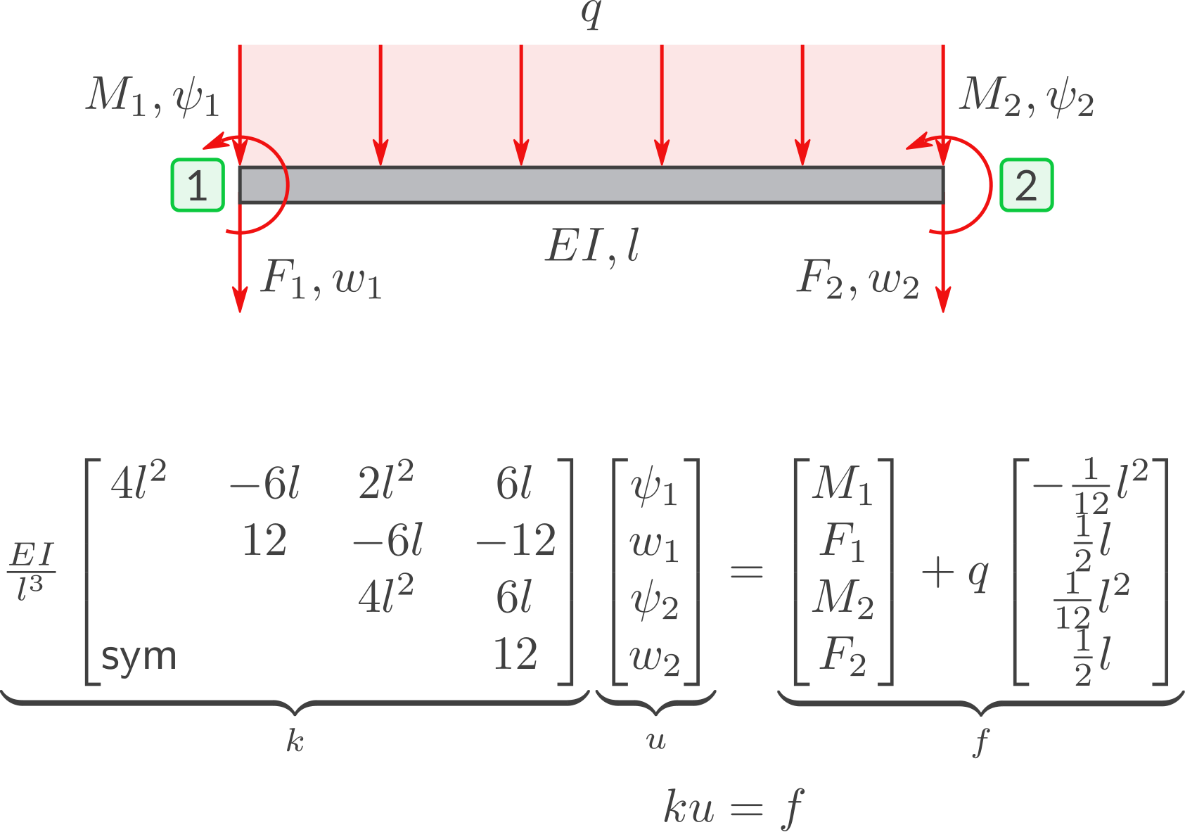
Andere Notationen
Es gibt verschiedene Notationen für diese Aussagen. Denn man kann in den Aussagen zum Linearen System die Symbole, die Zählrichtungen und die Reihenfolge wählen.
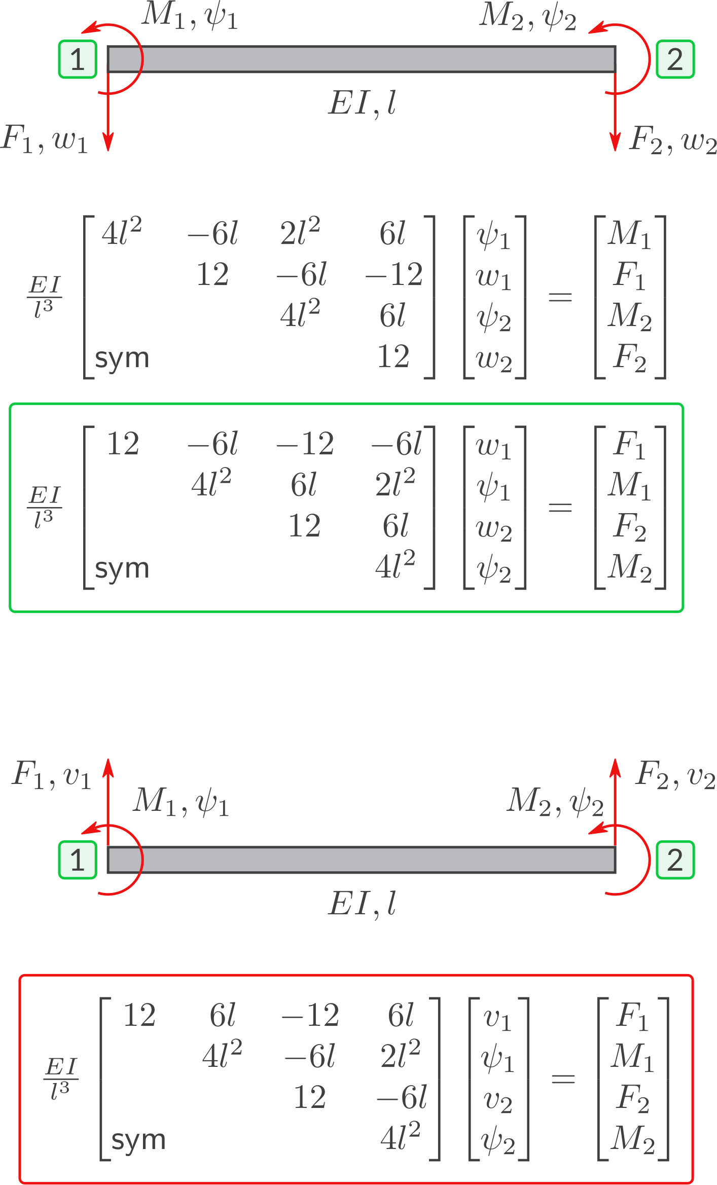
Grüner Kasten: Reihenfolge wie bei Dr. Bernd Klein. Roter Kasten: Symbole, Zählrichtungen und Reihenfolge wie bei Dr. Manfred Hahn.
Umformung des Gleichungssystems in Matrix-Schreibweise. Ausgangspunkt ist: Reihenfolge der Aussagen ändern liefert: Umbenennung der Symbole liefert: Minuszeichen in die Matrix bringen liefert: Multiplizieren der 1. und 3. Zeile mit -1 liefert:
Nachfolgend ein Programm, dass Sie ausführen können: Auf dem PC z.B. mit Anaconda. Im Browser (online) in drei Schritten: Copy: Source Code in die Zwischenablage kopieren. Paste: Source Code als Python-Notebook einfügen z.B. auf: JupyterLab oder Play: Ausführen. Statt SymPy lieber anderes CAS (Computeralgebrasystem) verwenden? Eine Auswahl verschiedener CAS gibt es hier.Details
SymPy
from sympy import *

EI, l = var("EI, l")

p1H, w1H, p2H, w2H = var("phi1, u1, phi2, u2")
M1H, F1H, M2H, F2H = var("B1, Q1, B2, Q2")
p1, w1, p2, w2 = var("psi1, w1, psi2, w2")
M1, F1, M2, F2 = var("M1, F1, M2, F2")

sub_list=[
    (p1,  p1H),
    (w1, -w1H),
    (p2,  p2H),
    (w2, -w2H),
    (M1,  M1H),
    (F1, -F1H),
    (M2,  M2H),
    (F2, -F2H),
    ]

u = Matrix([p1, w1, p2, w2])
f = Matrix([M1, F1, M2, F2])

def K(EI, l):
    # l = Element length
    l2, l3 = l*l, l*l*l
    K = EI/l3
    K *= Matrix([
        [  4*l2 ,  -6*l ,  2*l2 ,   6*l  ],
        [ -6*l  ,  12   , -6*l  , -12    ],
        [  2*l2 ,  -6*l ,  4*l2 ,   6*l  ],
        [  6*l  , -12   ,  6*l    , 12   ],
        ])
    return K

print("\nStandard Notation with EI/l³ omitted:")
K = K(EI, l)
fac = EI/(l**3)
pprint(K/fac)
pprint(u)
pprint(f)

pprint("\n1. Change Order:")
def swap(K, u, f, n, m):
    n = n-1
    m = m-1
    K.row_swap(n,m)
    K.col_swap(n,m)
    u.row_swap(n,m)
    f.row_swap(n,m)

# Shift to Hahn Notation:
swap(K, u, f, 1, 2)
swap(K, u, f, 3, 4)
pprint(K/fac)
pprint(u)
pprint(f)

pprint("\n2. Substitute Symbols in u and f:")
u = u.subs(sub_list)
f = f.subs(sub_list)
pprint(u)
pprint(f)

pprint("\n3. Move Negative Signs of u into Matrix:")
K.col_op(0, lambda i, j: i*(-1))
K.col_op(2, lambda i, j: i*(-1))
u.row_op(0, lambda i, j: i*(-1))
u.row_op(2, lambda i, j: i*(-1))
pprint(K/fac)
pprint(u)

pprint("\n4. Multiply Row 1 and 3 by -1:")
K.row_op(0, lambda i, j: i*(-1))
K.row_op(2, lambda i, j: i*(-1))
f.row_op(0, lambda i, j: i*(-1))
f.row_op(2, lambda i, j: i*(-1))
pprint(K/fac)
pprint(f)
Standard Notation with EI/l³ omitted:
⎡   2           2     ⎤
⎢4⋅l   -6⋅l  2⋅l   6⋅l⎥
⎢                     ⎥
⎢-6⋅l   12   -6⋅l  -12⎥
⎢                     ⎥
⎢   2           2     ⎥
⎢2⋅l   -6⋅l  4⋅l   6⋅l⎥
⎢                     ⎥
⎣6⋅l   -12   6⋅l   12 ⎦
⎡ψ₁⎤
⎢  ⎥
⎢w₁⎥
⎢  ⎥
⎢ψ₂⎥
⎢  ⎥
⎣w₂⎦
⎡M₁⎤
⎢  ⎥
⎢F₁⎥
⎢  ⎥
⎢M₂⎥
⎢  ⎥
⎣F₂⎦

1. Change Order:
⎡ 12   -6⋅l  -12  -6⋅l⎤
⎢                     ⎥
⎢         2          2⎥
⎢-6⋅l  4⋅l   6⋅l  2⋅l ⎥
⎢                     ⎥
⎢-12   6⋅l   12   6⋅l ⎥
⎢                     ⎥
⎢         2          2⎥
⎣-6⋅l  2⋅l   6⋅l  4⋅l ⎦
⎡w₁⎤
⎢  ⎥
⎢ψ₁⎥
⎢  ⎥
⎢w₂⎥
⎢  ⎥
⎣ψ₂⎦
⎡F₁⎤
⎢  ⎥
⎢M₁⎥
⎢  ⎥
⎢F₂⎥
⎢  ⎥
⎣M₂⎦

2. Substitute Symbols in u and f:
⎡-u₁⎤
⎢   ⎥
⎢φ₁ ⎥
⎢   ⎥
⎢-u₂⎥
⎢   ⎥
⎣φ₂ ⎦
⎡-Q₁⎤
⎢   ⎥
⎢B₁ ⎥
⎢   ⎥
⎢-Q₂⎥
⎢   ⎥
⎣B₂ ⎦

3. Move Negative Signs of u into Matrix:
⎡-12  -6⋅l   12   -6⋅l⎤
⎢                     ⎥
⎢        2           2⎥
⎢6⋅l  4⋅l   -6⋅l  2⋅l ⎥
⎢                     ⎥
⎢12   6⋅l   -12   6⋅l ⎥
⎢                     ⎥
⎢        2           2⎥
⎣6⋅l  2⋅l   -6⋅l  4⋅l ⎦
⎡u₁⎤
⎢  ⎥
⎢φ₁⎥
⎢  ⎥
⎢u₂⎥
⎢  ⎥
⎣φ₂⎦

4. Multiply Row 1 and 3 by -1:
⎡12   6⋅l   -12   6⋅l ⎤
⎢                     ⎥
⎢        2           2⎥
⎢6⋅l  4⋅l   -6⋅l  2⋅l ⎥
⎢                     ⎥
⎢-12  -6⋅l   12   -6⋅l⎥
⎢                     ⎥
⎢        2           2⎥
⎣6⋅l  2⋅l   -6⋅l  4⋅l ⎦
⎡Q₁⎤
⎢  ⎥
⎢B₁⎥
⎢  ⎥
⎢Q₂⎥
⎢  ⎥
⎣B₂⎦
Wie beim Stab-Element lässt sich die Knoten-Reihenfolge vertauschen, ohne dass sich die Einträge der Steifigkeitsmatrix ändern: Zugehörige erweiterte Steifigkeitsmatrizen:Details zur Wahl der Knoten-Reihenfolge
Erweiterte Steifigkeitsmatrix
Die erweiterte Element-Steifigkeitsmatrix bietet den Vorteil, dass die Freiheitsgrade \((\psi_1, w_1, \psi_2, w_2)\) sichtbar sind, auf die sich die Einträge der Steifigkeitsmatrix beziehen.
Interpolation
\(N_1, N_2, N_3, N_4, N_5\) sind die dimensionslosen Interpolationsfunktionen:
Ableitungen nach \(x\):
Ableitungen nach \(\xi\):
Querverschiebung w
Interpolierte Querverschiebung in Matrix-Schreibweise:
Bemerkung
Eine \(1 \times 5\)-Matrix multipliziert mit einer \(5 \times 1\)-Matrix ergibt eine \(1 \times 1\)-Matrix, also eine Zahl.
Man kann das Produkt auch so schreiben:
\[\begin{split}w &= \underbrace{ \begin{bmatrix} \psi_1 & w_1 & \psi_2 & w_2 & q \end{bmatrix} }_{1 \times 5} \underbrace{ \begin{bmatrix} l N_1 \\ N_2 \\ l N_3 \\ N_4 \\ \tfrac{l^4}{B} N_5 \end{bmatrix} }_{5 \times 1} \\ &= \underbrace{ \begin{bmatrix} l N_1 & N_2 & l N_3 & N_4 & \tfrac{l^4}{B} N_5 \end{bmatrix} }_{1 \times 5} \underbrace{ \begin{bmatrix} \psi_1 \\ w_1 \\ \psi_2 \\ w_2 \\ q \end{bmatrix} }_{5 \times 1}\end{split}\]\(w\) ist von der Ordnung \(\xi^4\).
Neigungswinkel ψ, Biegemoment M, Querkraft Q
Mit \(\psi=-w'\) und \(M = - B w''\) und \(Q = - B w'''\) gilt:
Graphische Darstellung
Schieberegler verschieben = Variieren des Knoten-Werts. In Legende Funktion klicken = Aus- und Einblenden des Funktionsgraphen. Horizontale Achse: Werte werden nach rechts größer - wie üblich. Vertikale Achse: Werte werden nach unten größer.Interaktive Diagramme
Äquivalente Knotenlasten
siehe equi
Lösung einiger Aufgaben
Nachfolgend ein Programm, dass Sie ausführen können: Auf dem PC z.B. mit Anaconda. Im Browser (online) in drei Schritten: Copy: Source Code in die Zwischenablage kopieren. Paste: Source Code als Python-Notebook einfügen z.B. auf: JupyterLab oder Play: Ausführen. Statt SymPy lieber anderes CAS (Computeralgebrasystem) verwenden? Eine Auswahl verschiedener CAS gibt es hier.SymPy
from sympy.physics.units import *
from sympy import *
# Units:
(mm, cm) = ( m/1000, m/100 )
kN = 10**3*newton
Pa = newton/m**2
MPa = 10**6*Pa
GPa = 10**9*Pa
deg = pi/180
half = S(1)/2
# Rounding:
import decimal
from decimal import Decimal as DX
from copy import deepcopy
def iso_round(obj, pv,
rounding=decimal.ROUND_HALF_EVEN):
import sympy
"""
Rounding acc. to DIN EN ISO 80000-1:2013-08
place value = Rundestellenwert
"""
assert pv in set([
# place value # round to:
"1", # round to integer
"0.1", # 1st digit after decimal
"0.01", # 2nd
"0.001", # 3rd
"0.0001", # 4th
"0.00001", # 5th
"0.000001", # 6th
"0.0000001", # 7th
"0.00000001", # 8th
"0.000000001", # 9th
"0.0000000001", # 10th
])
objc = deepcopy(obj)
try:
tmp = DX(str(float(objc)))
objc = tmp.quantize(DX(pv), rounding=rounding)
except:
for i in range(len(objc)):
tmp = DX(str(float(objc[i])))
objc[i] = tmp.quantize(DX(pv), rounding=rounding)
return objc
a, c, l, q, F, M, EI = var("a, c, l, q, F, M, EI")
quants = False
# quants = True
# sublist=[
# ( M, 10 *newton*m ),
# ( a, 1 *m ),
# ( EI, 200*GPa * 2*mm*6*mm**3/ 12 ),
# ]
def K(EI, l):
# l = Element length
l2, l3 = l*l, l*l*l
K = EI/l3
K *= Matrix([
[ 4*l2 , -6*l , 2*l2 , 6*l ],
[ -6*l , 12 , -6*l , -12 ],
[ 2*l2 , -6*l , 4*l2 , 6*l ],
[ 6*l , -12 , 6*l , 12 ],
])
return K
def K2(EI, l):
# l = Element length
l2, l3 = l*l, l*l*l
K = EI/l3
K *= Matrix(
[
[ 4*l2 , -6*l , 2*l2 , 6*l , 0 , 0 ],
[ -6*l , 12 , -6*l , -12 , 0 , 0 ],
[ 2*l2 , -6*l , 8*l2 , 0 , 2*l2 , 6*l ],
[ 6*l , -12 , 0 , 24 , -6*l , -12 ],
[ 0 , 0 , 2*l2 , -6*l , 4*l2 , 6*l ],
[ 0 , 0 , 6*l , -12 , 6*l , 12 ],
]
)
return K
def Fq(l):
return q*l/2
def Mq(l):
return q*l*l / 12
p0,w0,p1,w1,p2,w2 = var("ψ₀,w₀,ψ₁,w₁,ψ₂,w₂")
M0,F0,M1,F1,M2,F2 = var("M₀,F₀,M₁,F₁,M₂,F₂")
# task = "5.7"
# task = "B2.A"
# task = "B2.B"
# task = "B2.C"
# task = "B2.D"
task = "B2.E"
# task = "B2.E-MIRROR"
# task = "B2.E-POINT"
# task = "B2.F"
# task = "B2.G"
# task = "B2.H"
# task = "B2.I"
# task = "B2.J"
pprint("\nTask: "+task)
if task == "5.7":
K = K(EI, a)
# 1 2
#
# M
# |------------------------------
# a Λ
M = var("M")
#
u = Matrix([ 0,0, p2,0 ])
f = Matrix([ M1,F1, M,F2 ])
unks = [ M1,F1, p2,F2 ]
elif task == "B2.A":
K = K2(EI, a)
# 0 1 2
# F1 F2
# |------------------------------
u = Matrix([ 0,0, p1,w1, p2,w2 ])
f = Matrix([ M0,F0, 0,F1, 0,F2 ])
unks = [ M0,F0, p1,w1, p2,w2 ]
elif task == "B2.B":
K = K(EI, a)
# 1 2
# qqqqqqqqqqqqqqqqqqqqqqqqqqqqq
# |------------------------------
# a Λ
#
u = Matrix([ 0,0, p2,0 ])
f = Matrix([ M1-Mq(a),F1+Fq(a), 0+Mq(a),F2+Fq(a) ])
unks = [ M1,F1, p2,F2 ]
elif task == "B2.C":
K = K2(EI, a/4)
# 0 1 2
# ◆ qqqqqqqqqqqqqqqqqqqqqqqqqqqq
# -------------------------------
# ◆ Λ
#
u = Matrix([ 0,w0, p1,w1, p2,0 ])
f = Matrix([M0-Mq(a/4),Fq(a/4), 0,2*Fq(a/4), Mq(a/4),F2+Fq(a/4) ])
unks = [ M0,w0, p1,w1, p2,F2 ]
elif task == "B2.D":
K = K(EI, a)
# 1 2
# F
# qqqqqqqqqqqqqqqqqqqqqqqqqqqqq
# ------------------------------|
# Λ a
# |
# | cw₁
#
u = Matrix([ p1,w1, 0,0 ])
f = Matrix([ 0-Mq(a),F+Fq(a), M2+Mq(a),F2+Fq(a) ])
# Spring instead of q:
# f = Matrix([ 0,F-c*w1, M2,F2 ])
unks = [ p1,w1, M2,F2 ]
elif task == "B2.E":
K = K2(EI, a)
Ml = -q*a*a / 12
Mr = q*a*a / 12
Fq = q*a/2
# 0 1 2
# qqqqqqqqqqqqqq
# |-----------------------------|
#
u = Matrix([ 0,0, p1,w1, 0,0 ])
f = Matrix([ M0,F0, Ml,Fq, M2+Mr,F2+Fq ])
unks = [ M0,F0, p1,w1, M2,F2 ]
elif task == "B2.E-MIRROR" or task == "B2.E-POINT":
K = K(EI, a)
Ml = -q*a*a / 12 / 2
Mr = q*a*a / 12 / 2
Fq = q*a/2 / 2
if task == "B2.E-MIRROR":
#
# 0 1
# q/2 q/2 q/2
# |---------------- Mirror Symm.: ψ1=0, F1=0
#
u = Matrix([ 0,0, 0,w1 ])
f = Matrix([ M0+Ml,F0+Fq, M1+Mr,0+Fq ])
unks = [ M0,F0, w1,M1 ]
elif task == "B2.E-POINT":
# 0 1
# -q/2 -q/2 -q/2
# |---------------- Point Symm.: w1=0, M1=0
#
u = Matrix([ 0,0, p1,0 ])
f = Matrix([ M0-Ml,F0-Fq, 0-Mr,F1-Fq ])
unks = [ M0,F0, p1,F1 ]
elif task == "B2.F":
K = K2(EI, a)
# 0 1 2
# qqqqqqqqqqqqqq
# ------------------------------|
# Λ
#
u = Matrix([ p0,0, p1,w1, 0,0 ])
f = Matrix([ 0-Mq(a),F0+Fq(a), 0+Mq(a),0+Fq(a), M2,F2 ])
unks = [ p0,F0, p1,w1, M2,F2 ]
elif task == "B2.G":
Mq1, Fq1 = -q/12*a*a, q/2*a
Mq2, Fq2 = -Mq1, Fq1
# 0 1 2
# qqqqqqqq
# |------------------------------
# 2a Λ a
#
u = Matrix([ 0,0, p1,0, p2,w2 ])
f = Matrix([ M0,F0, Mq1,Fq1+F1, Mq2,Fq2 ])
unks = [ M0,F0, p1,F1, p2,w2 ]
# Elem. 1
l = 2*a
l2 = l*l
l3 = l*l*l
K = EI/l3 * Matrix(
[
[ 4*l2 , -6*l , 2*l2 , 6*l , 0 , 0 ],
[ -6*l , 12 , -6*l , -12 , 0 , 0 ],
[ 2*l2 , -6*l , 4*l2 , 6*l , 0 , 0 ],
[ 6*l , -12 , 6*l , 12 , 0 , 0 ],
[ 0 , 0 , 0 , 0 , 0 , 0 ],
[ 0 , 0 , 0 , 0 , 0 , 0 ],
]
)
# Elem. 2
l = a
l2 = l*l
l3 = l*l*l
K += EI/l3 * Matrix(
[
[ 0 , 0 , 0 , 0 , 0 , 0 ],
[ 0 , 0 , 0 , 0 , 0 , 0 ],
[ 0 , 0 , 4*l2 , -6*l , 2*l2 , 6*l ],
[ 0 , 0 , -6*l , 12 , -6*l , -12 ],
[ 0 , 0 , 2*l2 , -6*l , 4*l2 , 6*l ],
[ 0 , 0 , 6*l , -12 , 6*l , 12 ],
]
)
elif task == "B2.H":
M, c = var("M, c")
Fc = c*w1
K = K2(EI, a/2)
# 0 1 2
# M M
# |------------------------------
# Λ
# | Fc = c w₁
# |
#
u = Matrix([ 0,0, p1,w1, p2,w2 ])
f = Matrix([ M0,F0, M,-Fc, M,0 ])
unks = [ M0,F0, p1,w1, p2,w2 ]
elif task == "B2.I":
K = K(EI, a/2)
# 1 2
# F/2
#
# ◆
# -------------------------------
# ◆ a/2 Λ
#
#
#
u = Matrix([ 0,w1, p2,0 ])
f = Matrix([ M1,F/2, 0,F2 ])
unks = [ M1,w1, p2,F2 ]
elif task == "B2.J":
K = K(EI, a)
# 1 2
# |
# | F
# V -M
# |------------------------------
# a Λ
#
#
#
# Equiv. Nodal Loads due to F:
M, F = var("M, F")
Me1, Fe1, Me2, Fe2 = -F*a/8, F/2, F*a/8, F/2
#
u = Matrix([ 0,0, p2,0 ])
f = Matrix([ M1+Me1,F1 + Fe1, -M+Me2,F2+Fe2 ])
unks = [ M1,F1, p2,F2 ]
eq = Eq(K*u , f)
sol = solve(eq, unks)
pprint("\nSolution")
pprint(sol)
exit()
for s in unks:
for tmp in [s, sol[s]]:
tmp = tmp.expand()
tmp = tmp.simplify()
pprint(tmp)
# pprint(latex(tmp,**kwargs))
pprint("\n")
if task =="5.7" and quants == True:
tmp = sol[s]
tmp = tmp.subs(sub_list)
if s == M1:
pprint("\nM1 / Nm:")
tmp /= newton*m
elif s == F1:
pprint("\nF1 / N:")
tmp /= newton
elif s == p2:
pprint("\np2 / rad (unrealistic task):")
tmp = tmp
elif s == F2:
pprint("\nF2 / N:")
tmp /= newton
tmp = iso_round(tmp,"1.0")
pprint(tmp)
if task == "B2.H":
pprint("\nw2 for ca³ = 10 EI:")
tmp = sol[w2]
tmp = tmp.subs(EI, c*a**3/10)
tmp = N(tmp,3)
pprint(tmp)
Task: B2.E

Solution
⎧                                  2             2           4          3   ⎫
⎪    -3⋅a⋅q       -13⋅a⋅q       5⋅a ⋅q      -11⋅a ⋅q        a ⋅q      -a ⋅q ⎪
⎨F₀: ───────, F₂: ────────, M₀: ──────, M₂: ─────────, w₁: ─────, ψ₁: ──────⎬
⎪       16           16           48            48         48⋅EI      96⋅EI ⎪
⎩                                                                           ⎭